How to Read a Stem Leaf Plot

Stalk and Leaf plots

In the last article, we looked at the histogram as a way of describing and understanding the trends in Quantitative Data. Let'due south look at some other kind of plot for describing Quantitative Information which is the Stem and Foliage plot. Information technology is an efficient manner of describing minor to medium data sets.

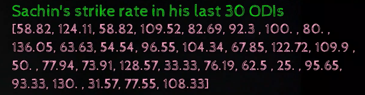
Allow's say we accept the data for the runs scored past Sachin in his last 30 ODIs.

Stem and Leafage plot represents every number/information item in the data(score in each lucifer in this instance) in two parts, one is called the stalk and the other is chosen the leaf

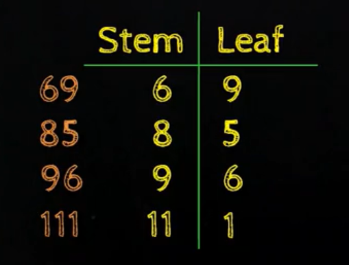
Let'southward take 1 number from the above dataset say 69, so in stem and leaf plot, what nosotros do typically is that we accept the last digit as the leafage and the other digit as the stalk. Let's take other values from the dataset equally well:

So, this is what the information would look like in a stem and leaf plot. The entire dataset in this tabular format would exist represented equally:

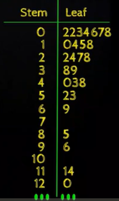
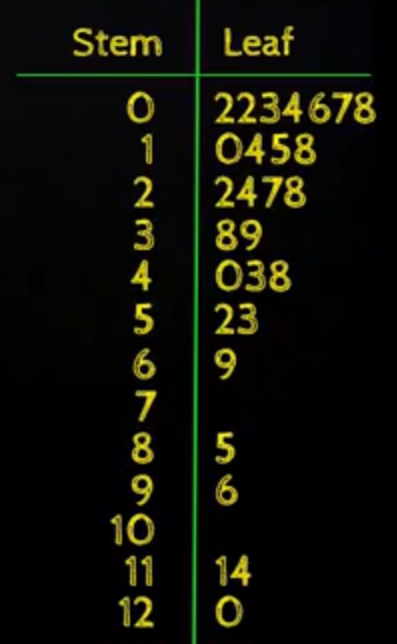
Let's sympathise this using the row having the Stem every bit 1, so we accept the Stalk every bit 1 and 0458 as the Leafage, what that means is that in the interval of 10 to 20, in that location are value 10, fourteen, xv, 18(i.e stem with each of private digits from the foliage), so that's this table captures.

At this point, information technology might be obvious that this is just like an inverted mode of showing a Histogram.

The first row that we run across essentially represents the interval 0 to x and nosotros accept the values in that interval which is the scores of 2, 2, three, iv, 6, seven, 8 and similarly, if we look at the 3rd row so it's the interval twenty to 30 and it has values 22, 24, 27, 28. So, that's how nosotros interpret this tabular format.

We could also apply Stalk and Leaf plot for continuous data where nosotros have fractional numbers, typically now this convention varies from place to identify, in many packages, it merely rounds off the number, so 58.ix would convert to 59, so those packages actually catechumen the continuous data to discrete data and with the discrete information we tin can draw the stem and foliage plot as discussed above.

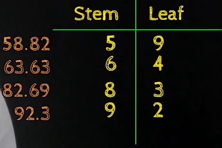
So, this tabular format actually looks similar a histogram in the sense that it conveys the same data for example the interval 20 to 30 contains ane value, the interval 30 to 40 contains 2 values, the interval 40 to fifty contains no values in the dataset, and so on.

Now ane question is what if we have larger values? Here in both the examples that we took, we had only two digit values and hence the decision was like shooting fish in a barrel to use one digit as the stalk and the other equally the leaf simply what if have larger values like in the below image?

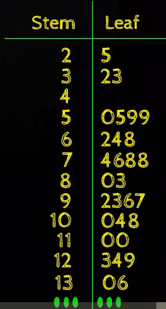
If nosotros have bigger values like 6 digit values, let's wait at what happens if we draw the stem and leaf plot as earlier where we proceed the terminal digit for the leafage and the remaining digits for the stem

This does not look very interesting as we tin't encounter very interesting patterns hither, and then if we wait at information technology as an inverted histogram, then we have the numbers on the 10-axis every bit 17952, 18059, and then on and each of these numbers has just i element inside information technology, information technology's just similar all the confined are of size ane and every bit nosotros know that having such kind of grade intervals typically does not help in getting interesting patterns from the data.

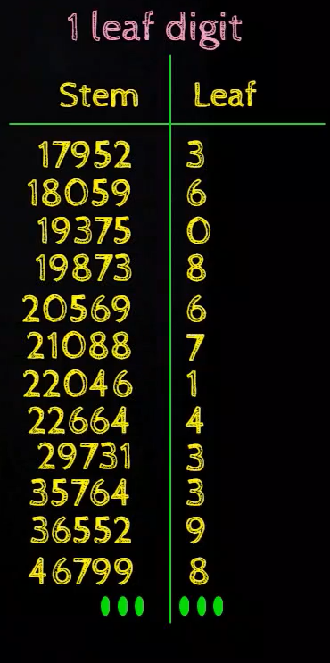
So, what we do in this case is that we cull the last 4 digits as the leaf and the first two digits every bit the stem

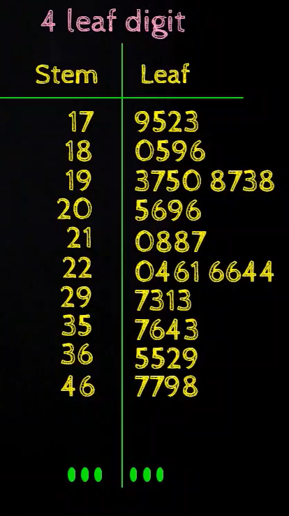
Now it looks like in the interval of 1700000 to 1800000, there is ane value which is 9523 so that'south 17900523, in the interval of nineteen lakhs to 20 lakhs there are two values i.eastward 19003750 and 19008738, then that'due south how we read this table.

So, if nosotros have larger values, we need to determine what kind of class interval makes sense(how many digits to consider as stem and how many as the leaf).

The central matter to annotation hither is that every row is 1 course interval and we write the value(s) in that class interval in the leaf office and at that place are multiple conventions hither: ane convention is that when nosotros have this large number of digits(similar the 6 digit information in the in a higher place example), then we simply decide what is okay for the stem, is it okay to have a 1 digit stalk or a 2 digit stem and nosotros put that in the stem column and and then we don't write out the entire value in leaf, just we just keep one digit there, so in the beneath image for the first row, we will just keep the digit 9 and it is understood that this is some value in 9000, then similarly for the 3rd row, we will proceed the value iii and 8 which is understood that this is some value in 3000 and 8000. At the same time, it does no impairment to keep the full value besides, so it depends on whether it'south becoming a scrap cumbersome and we just desire to retain just ane digit and have the interpretation that whatever digit is in that location, we multiply it by 1000 because we are curtailing the concluding three digits of the number.

The key matter here is that instead of just drawing bars, we are actually writing down the values, then nosotros are having more details here as compared to the histogram.

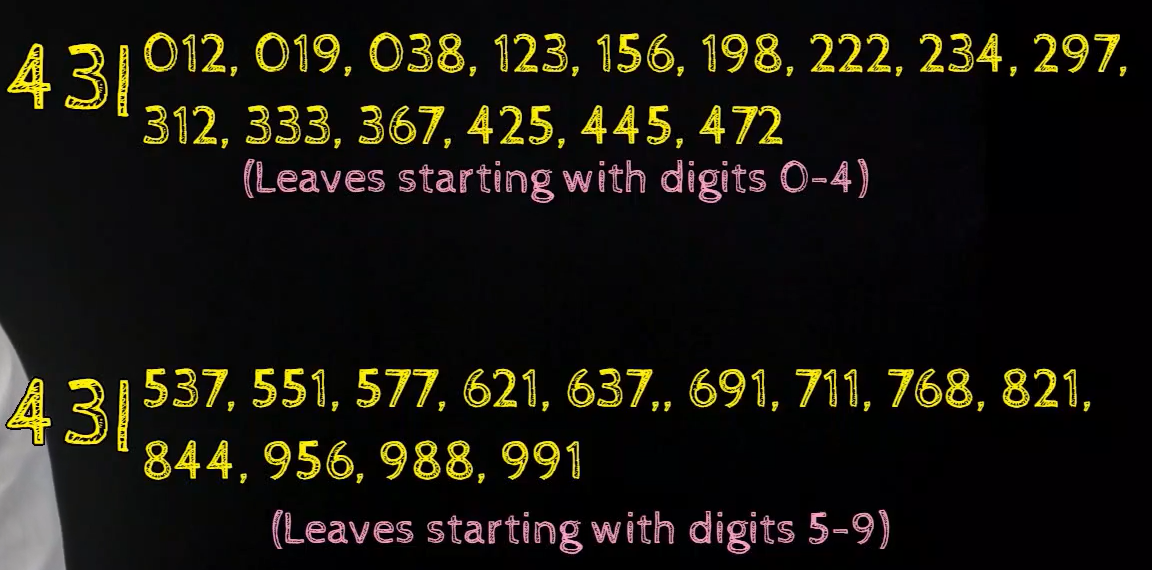
What if a row has many values?

Now sometimes what happens is that say we take a stem of 43 as depicted in the beneath image and it has a large number of values, it has values 012, 019 all the mode upwardly to 472 and and then 537, 551, 577, all the manner upwards to 991. In such cases, we split up this row into two parts, so we write the stalk 43 twice and the first row will just contain the leaves starting from 0 to 4 and the second row will contain the leaves starting from v to 9.

Stem Plot vs Histogram

Here is the stem and leaf plot and the histogram for the runs scored by Sachin in 30 ODIs and we have the interval 0 to 10, 10 to 20, and then on in the histogram. Similarly, we have the intervals 0, 1, 2, and then on where we know that the interval 2 or the value 2 corresponds to the interval 20 to 30

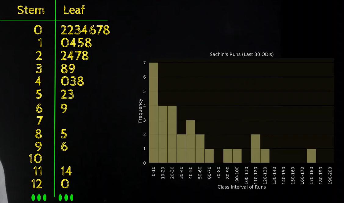
At present if we remember of the Stem and Leaf plot as the inverted histogram, we have these confined throughout, it volition look similar:

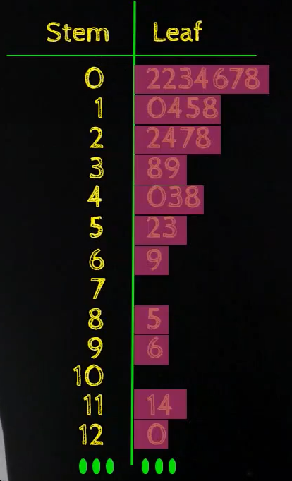
This has the added advantage that nosotros are at present also zooming into the bar, in the histogram, we don't know what are the individual values but here nosotros have the access to the private values too and that's how Stem and Leaf plot is different from a histogram because information technology has more details and whatsoever patterns nosotros could find from a histogram which in the above case is that there are a lot of values in the earlier interval and very few values in the later class interval, the same pattern can as well be understood from a stalk and leaf plot.

Stem and Leaf plot is not preferred for large datasets. Hither is another dataset where we have a large number of values, so here nosotros can't actually make sense of all the zoomed-in values that we have, nosotros just care for this as a long bar and not really be able to see all the values within it

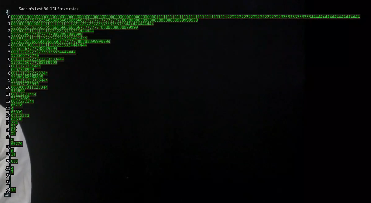
When we have really big datasets, a stem and foliage plot is non preferred, nosotros would rather have a histogram.

The reward of having a stem and leaf plot is that we have these values inside which makes information technology very like shooting fish in a barrel to spot certain patterns within each class interval.

For example, if nosotros look at the course interval 60 to 70 here, we meet that a lot of values there are 64, so the value 64 appears very frequently as opposed to any other value in that row which is 61 or 65 or 67 or 69.

So, such patterns like what is happening inside the form interval become obvious in a stem and leafage plot.

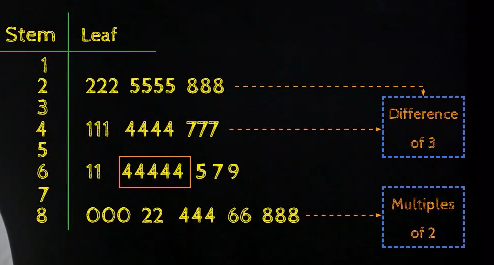
In the above paradigm, nosotros can also see that the row corresponding to 80 has all numbers which are multiples of 2.

And similarly, if nosotros look at the rows corresponding to interval 20 and forty, we see that the difference between the values is iii. Then, nosotros have a value 41, then we have a value 44, then 47 and the same is true for row number ii or the interval twenty–30.

So, such types of patterns becomes clear in a stalk and leaf plot because nosotros take this zoomed in version of the data where within the bars, we are also seeing the values while non missing any of the other details that nosotros meet in a histogram, the overall trend is still visible here simply the merely upshot is that we can practice this for minor datasets, for large datasets, its just too much information and nosotros won't be able to make sense of zoomed in data that we have in the large datasets.

Then, we also take back to dorsum stem and leaf plots which allow us to compare two datasets. Say we want to compare the ODI scores of Sachin with his Test scores, sample data looks like the below

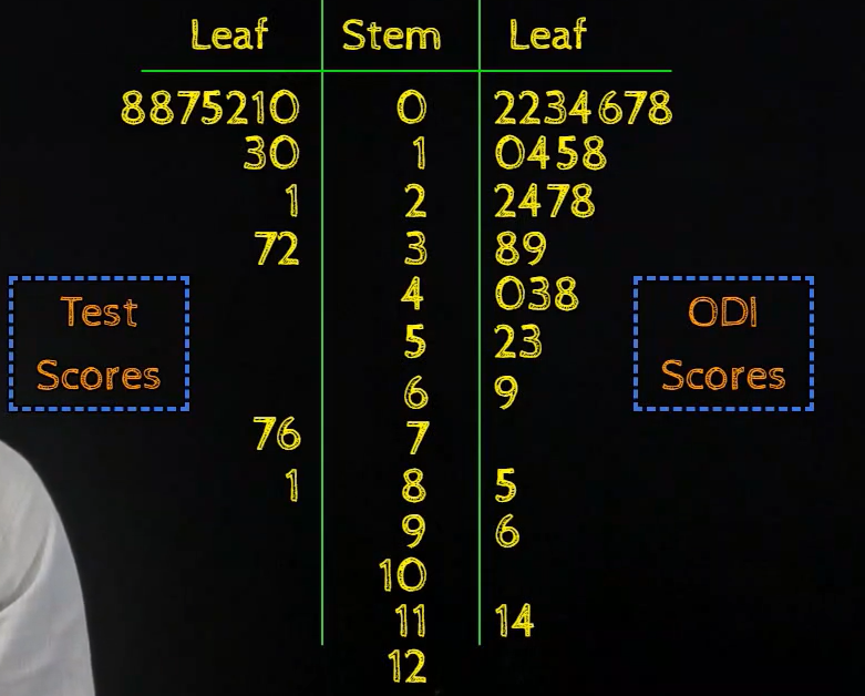
Here, once again we see that in that location are a lot of values in the lower range, so there are a lot of values below twenty.

So, a back to dorsum stalk and leafage plot helps us to compare two datasets.

mccannwarl1966.blogspot.com

Source: https://prvnk10.medium.com/stem-and-leaf-plot-2d2a8907f757

Share this post